
Verification or calibration intervals are often the subject of much debate. Should equipment systematically be verified or calibrated every year?
Unfortunately, there are only two possible answers to this question:
The first is often imposed by the test standard and/or the
equipment calibration method, which may state, for example, that the calibration
interval must not exceed 12 months. From an assessor’s perspective, the drift
must not be too significant, as they could consider that the equipment is
not under control, unless this exceedance is justified, for example, through
a documented deviation or waiver.
It should be noted that some laboratories have asked the notified body for authorization to extend the traceability interval for certain items of equipment because the number of tests performed did not justify the cost of annual traceability services.
The interval was therefore extended, and these items of equipment are now calibrated every two years. Could the potential drift penalize the test results? I do not think so, provided, of course, that periodic checks are implemented to control the equipment’s response.
The second option, which offers more flexibility, consists in selecting an appropriate traceability interval for each item of equipment when no interval is imposed by standards.
This is the choice of interval that will be developed in the content below.
As a general rule, the traceability interval is based on several criteria:
- The client’s requirement for accurate, reliable, and high-quality measurements.
- The equipment drift observed over previous years.
- Common practices within the profession for similar equipment.
- The need to reduce calibration costs, a requirement generally driven by management
due to increasing external costs that reduce margins.
Meeting all of these criteria is often difficult. Calibration intervals must be adjusted in a way that supports both the quality of the services provided and cost-reduction objectives.
Basic Concept
The reader may also refer to the document “Optimization of Calibration Periodicities:
The Opperet Method” available from the CFM.
The concept presented in this document is not based on that method.
The extent to which the value of a given parameter can be known at the time
of calibration is determined by a number of variables. These include the calibration
uncertainty of the equipment, the accuracy with which the measurements can
be performed, the stability of the measurement process, the skill of the person
performing the calibration, and so on.
Immediately after calibration, knowledge of the value of this parameter is
associated with a range of values, or function, that can be fairly well defined.
After a certain period of time, this function becomes less accurate. Due to
the random processes inherent in testing, as well as the diversity of measurements
and the equipment environment, the parameter values tend to vary randomly.
This random variation propagates the distribution of the original parameter
values, and over time, the spread of the values increases.
Thus, the uncertainty surrounding the value of the calibrated parameter increases
as time elapses since the last calibration.

Laboratories primarily concerned with measurement integrity tend to use calibration
intervals that are often shorter, which is not necessarily economically justifiable.
Conversely, in laboratories that are mainly concerned with the economic aspect
rather than measurement integrity, calibration intervals often tend to be
longer, which may prove detrimental with respect to measurement uncertainty.
Calibration Interval Analysis System
The objective of any calibration interval analysis system should be to keep
the cost for each interval to a minimum.
This requirement, when combined with the need to achieve measurement reliability
objectives, leads to the following objectives:
- Establishing appropriate measurement reliability objectives
- Adjusting intervals to achieve reliability objectives
- Using algorithms and methods that allow appropriate intervals to be obtained
as quickly as possible
- Determining calibration intervals with minimal human intervention
The implementation of such a strategy requires the following elements:
• Data collection and storage, allowing the time-dependent increase in measurement
uncertainty to be inferred.
• Reliability modeling, using a statistical model to support the determination
of calibration intervals.
• Statistical analysis of calibration results. Statistical methods are used
to adjust reliability models to the data and to identify abnormal or exceptional
circumstances.
• Cost/benefit analysis. These methods make it possible to optimize calibration
frequency and, consequently, external costs.
• Personnel requirements. Statistical knowledge is preferable for personnel
responsible for determining calibration intervals.
• Training and communication. A good understanding of the principles governing
the increase in uncertainty, as well as an appreciation of how calibration
data are used to establish and adjust intervals, is necessary to promote data
accuracy.
Reliability Modeling of Equipment
The increase in the measurement uncertainty of a parameter at time t is described
by its statistical probability density function f(x(t)).
Considering the representation of measurement reliability, R(t), at time t,
and the tolerance limits L1 and L2 of the parameter, the relationship between
measurement reliability and f(x(t)) is given by the integral:

Measurement reliability is the probability that a parameter operates in an out-of-tolerance condition.
At a given time t elapsed since calibration, the probability can be sampled by performing a number of calibrations n(t). If the number of calibrations for which the parameter was found to be within tolerance is represented by g(t), then the measurement reliability at time t is:

Given an exponential distribution, the probability that an instrument remains
within tolerance over a time interval t
(1) R(There was no problem before t)=R
Let’s take a numerical example to explain the approach, assuming that at
t = 1 week, g(t)/n(t)=R
|
Week number in the year (t) |
Number of calibrations performed n(t) |
Number of calibrations within tolerances g(t) |
Measured reliability R(t) |
|
1 |
1 |
1 |
1,00 |
|
4 |
6 |
6 |
1,00 |
|
9 |
5 |
5 |
1,00 |
|
12 |
4 |
4 |
1,00 |
|
20 |
4 |
3 |
0,75 |
|
27 |
6 |
4 |
0,66 |
|
38 |
6 |
3 |
0,50 |
|
49 |
5 |
2 |
0,40 |
Simple approach:
Let us start with calculations that can be applied without any specific expertise:
We will determine the failure rate of our equipment, i.e. λ
by calculating the total number of calibrations:N, and the
total number of calibrations: G, found to be within tolerance.
Let’s run the calculations:N=∑n=(1+6+5+4+4+6+6+5)=37 et G=∑g=(1+6+5+4+3+4+3+2)=28.
Ensuite, nous allons calculés la moyenne du temps T des étalonnages, il s'agit d'une moyenne pondérée qui se calcule avec la formule:
T=1/Nx∑tjnj=1/37x(1x1+4x6+9x5+12x4+20x4+27x6+38x6+49x5)=1/37x833=22,5 semaines
Next, we will calculate the average calibration time T. This is a weighted average calculated using the following formula:
R(no failure before T)≈G/N≈28/37≈0,75
Using the exponential equation (1), we can write: G/N=exp-λoT where λ₀ is the estimate of λ
We can therefore conclude: λ
Therefore: R(t)=exp-0,0124t

More scientific approach:
Several models are used to represent the evolution of uncertainty over time, such as exponential models, Weibull models, and others,..
R(t)=Roexp-λt is the exponential model characterized by R₀ and λ: R₀ is the reliability at t = 0, and λ is the failure rate..
It is used when the out-of-tolerance calibration rate remains constant over time (see the different modeling approaches at the bottom of the page).
We need to model the function R(t) = f(t) in Excel. Using an exponential law such as R(t) = R₀ exp(-λt), we can see that λ₀ = 0.017. The more simplified estimate is not bad either, with a deviation of 0.0017.
In the constraints, Excel must be forced to pass through 1 so that R₀ is equal to 1.
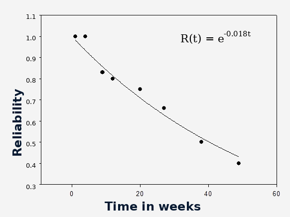
Please note that, for certain types of modeling, Excel will be limited for several reasons: the more complex formula may not be available among the proposed options, Excel does not iterate the model to obtain a more accurate estimate, and boundary conditions cannot always be imposed. In such cases, more powerful software, such as SigmaPlot, for example, will need to be used.
But what do we do with this equation?
Calculation of confidence limits with a 95% probability:
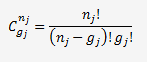
I will not go into the mathematical derivation of the formula used to estimate the maximum probability based on the probability that an instrument remains compliant after a period of use t.
I will only provide the basic formula, which is based on a binomial probability distribution::

avec
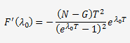
The maximum probability is obtained by differentiating the probability of R and using an estimate of λ based on λ₀.
L'erreur sur λ
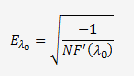
The error on λ₀ is obtained from the second derivative of F′(λ₀):


K is the coverage factor, which will be taken as equal to 1.96 for a 95% confidence level.
Passons à quelques applications numériques et calculons F'(λ

Eλo =0,000746
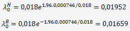
Let’s move on to a few numerical examples and calculate F′(λ₀)
On peut en déduire que:

This suggests that:

The error in t₀ can be estimated by:
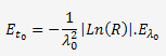
The lower and upper limits of t₀ are given by:

Let’s move on to a few numerical applications and calculate t₀ for a reliability of R = 0.85:
We know that: λ


For a reliability of R = 0.85, the verification or calibration interval with a 95% probability is 9 weeks, with a general tolerance of 1.5 weeks.
The same calculations can, of course, be performed using λ, but a program will be required to determine the probability of L according to::
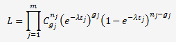
The results will be slightly different, but the estimate using λ0 is sufficiently accurate.
Weibull model

where β is the shape factor