Statistical Controls
Statistical inspection differs from 100% inspection, which is often costly but remains mandatory when the results of statistical inspection are not satisfactory, since the parts must then be sorted in order to remove the nonconforming ones, or when the product is critical with regard to personal safety.
Statistical inspection, also referred to as sampling inspection, is particularly suitable for tests that may damage the item being inspected, as well as for large population sizes, since it is easier to inspect a few items out of 1,000 or 10,000.
Two types of risk are distinguished in statistical inspection:
The customer’s risk, also called the consumer’s risk, denoted β: this is the
probability of accepting a bad lot, i.e., a lot that should have been rejected.
The supplier’s risk, also called the producer’s risk, denoted α: this is the
probability of having a good lot rejected.
| Matrix | The lot is conforming | The lot is nonconforming |
| Rejection | α Risk | Correct decision |
| Acceptance | Correct decision | β Risk |
The challenge therefore lies in selecting the appropriate sampling plan with respect to the available population.

A laboratory performs thickness measurements on 25 coated parts, each with a gold deposit of approximately 1.5 µm. For each part, 5 measurements are performed by coulometric testing.
The tolerance is ±0.5 µm.
We want to establish statistical process control using the mean x̄ and the range R.
| Nb | 1 | 2 | 3 | 4 | 5 | Average=x̄ | Max-Min=R̄ |
| 1 | 1,3235 | 1,4128 | 1,6744 | 1,4573 | 1,6914 | 1,5119 | 0,3679 |
| 2 | 1,4314 | 1,3592 | 1,6075 | 1,4666 | 1,6109 | 1,4951 | 0,2517 |
| 3 | 1,4284 | 1,4871 | 1,4932 | 1,4324 | 1,5674 | 1,4817 | 0,1390 |
| 4 | 1,5028 | 1,6352 | 1,3841 | 1,2831 | 1,5507 | 1,4712 | 0,3521 |
| 5 | 1,5604 | 1,2735 | 1,5265 | 1,4363 | 1,6441 | 1,4882 | 0,3706 |
| 6 | 1,5955 | 1,5451 | 1,3574 | 1,3281 | 1,4198 | 1,4492 | 0,2674 |
| 7 | 1,6274 | 1,5064 | 1,8366 | 1,4177 | 1,5144 | 1,5805 | 0,4189 |
| 8 | 1,4190 | 1,4303 | 1,6637 | 1,6067 | 1,5519 | 1,5343 | 0,2447 |
| 9 | 1,3884 | 1,7277 | 1,5355 | 1,5176 | 1,3688 | 1,5076 | 0,3589 |
| 10 | 1,4039 | 1,6697 | 1,5089 | 1,4627 | 1,5220 | 1,5134 | 0,2658 |
| 11 | 1,4158 | 1,7667 | 1,4278 | 1,5928 | 1,4181 | 1,5242 | 0,3509 |
| 12 | 1,5821 | 1,3355 | 1,5777 | 1,3908 | 1,7559 | 1,5284 | 0,4204 |
| 13 | 1,2856 | 1,4106 | 1,4447 | 1,6398 | 1,1928 | 1,3947 | 0,4470 |
| 14 | 1,4951 | 1,4036 | 1,5893 | 1,6458 | 1,4969 | 1,5261 | 0,2422 |
| 15 | 1,3589 | 1,2863 | 1,5996 | 1,2497 | 1,5471 | 1,4083 | 0,3499 |
| 16 | 1,5747 | 1,5301 | 1,5171 | 1,1839 | 1,8662 | 1,5344 | 0,6823 |
| 17 | 1,3680 | 1,7269 | 1,3957 | 1,5014 | 1,4449 | 1,4874 | 0,3589 |
| 18 | 1,4163 | 1,3864 | 1,3057 | 1,6210 | 1,5573 | 1,4573 | 0,3153 |
| 19 | 1,5796 | 1,4185 | 1,6541 | 1,5116 | 1,7247 | 1,5777 | 0,3062 |
| 20 | 1,7106 | 1,4412 | 1,2361 | 1,3820 | 1,7601 | 1,5060 | 0,5240 |
| 21 | 1,4371 | 1,5051 | 1,3485 | 1,5670 | 1,4880 | 1,4691 | 0,2185 |
| 22 | 1,4338 | 1,5936 | 1,6583 | 1,4973 | 1,4720 | 1,5390 | 0,1863 |
| 23 | 1,5917 | 1,4333 | 1,5551 | 1,5295 | 1,6866 | 1,5592 | 0,2533 |
| 24 | 1,6399 | 1,5243 | 1,5705 | 1,5563 | 1,5530 | 1,5688 | 0,1156 |
| 25 | 1,5797 | 1,3663 | 1,6240 | 1,3732 | 1,6887 | 1,5264 | 0,3224 |
We will calculate the mean of the means using the following equation:
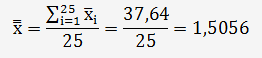
We will calculate the average range using the following equation:
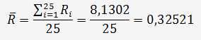
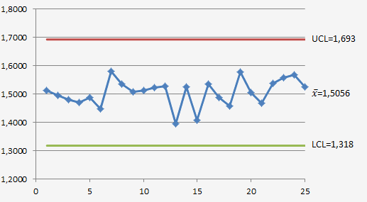
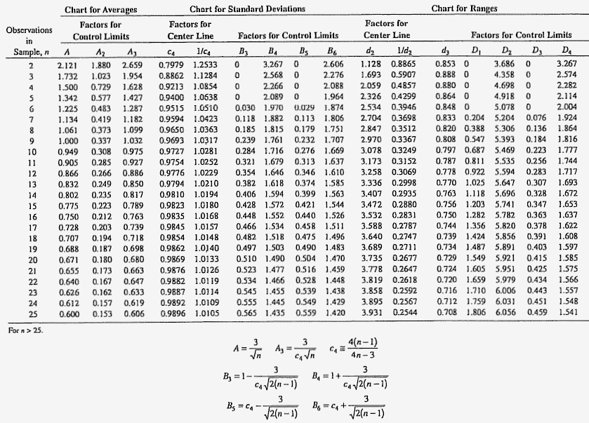
When using an X-bar control chart, the upper and lower control limits are calculated as follows:
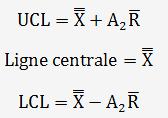
The coefficient A
UCL=1,5056+0,577.0,32521=1,693
LCL=1,5056-0,577.0,32521=1,318
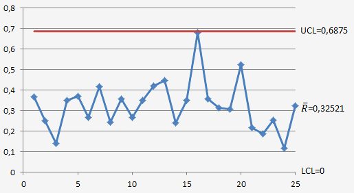
If a range control chart is used, the upper and lower limits are calculated as follows:
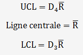
The coefficients D
UCL=2,114.0,32521=0,6875
LCL=0
We will assess the process capability:
The average x̄ and R charts provide information about process performance and capability
The process standard deviation, expressed in µm, can be estimated using the following relationship:

The standard deviation calculated from the 125 values is 0.1332 µm.
We will estimate the fraction of nonconforming thickness measurements:
Assuming that the measured thickness values follow a normal distribution, we know the mean thickness (1.5056 µm) and the process tolerance (±0.5 µm, i.e., Maximum = 2.0 µm and Minimum = 1.0 µm).
The following probability must be calculated:
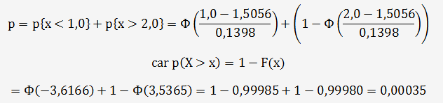
p = 0.035%, i.e. 350 ppm (parts per million), represents the probable nonconformity rate.
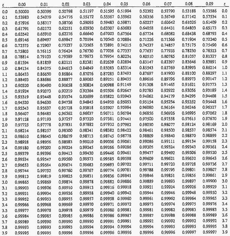
he values of Φ (the cumulative distribution function) are given in the table below:
We can also provide process capability using the Six Sigma method:
We know the process standard deviation: 0.1398 µm, and the process tolerance: ±0.5 µm, i.e. Maximum = USL = 2.0 µm and Minimum = LSL = 1.0 µm

Cp is greater than 1, as shown in Figure A.
We can estimate the percentage of the specification range that is being used:
We know the process capability: 1.192, and it is calculated using the following equation:
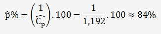
The process consumes 84% of the tolerance range.
We have seen that, for a percentage of 84%, the probability of obtaining nonconforming thickness values is 0.035%.
If we had had a Cp = 1 (diagram b), the process would use 100% of the tolerance range. The process standard deviation would therefore be 0.166 µm, and the probability of obtaining nonconforming thickness values would be 0.27% — i.e. 2,700 ppm, based on the probability calculation.
In the case of a Cp < 1 (diagram c), the process would use more than 100% of the tolerance range. The process standard deviation would therefore be greater than 0.166 µm, and the number of nonconforming thickness values would increase significantly.
Statistically, Cp should be greater than 1.33. This corresponds to 75% of the tolerance range and a probable nonconformity rate of 0.004%, under the conditions of this example, of course.

Burr’s constants for control chart limits
The Φ values correspond to the cumulative distribution function