
The ANOVA method (ANalysis Of VAriance) is preferred over the range and average method. It quantifies the interaction between repeatability and reproducibility and is considered more accurate than the range and average method.
To quantify repeatability and reproducibility using the ANOVA method, several parts, one measuring system, operators, and measurements are required.
The recommended method is to use 10 parts, 3 operators, and 3 measurement trials, for a total of 90 measurements.
The ANOVA method uses statistical techniques, such as the F-test, to analyze the effects of the different factors involved in the measurements.
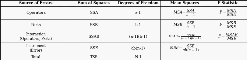
a = number of operators = 3,
b = number of parts = 10,
n = number of tests = 3
N = total number of tests (abn) = 90
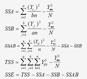
The measurement system repeatability, EV, is given by the following formula:

The AV reproducibility of the measurement system is given by the following formula:
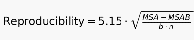
The interaction between the operators and the parts is given by :
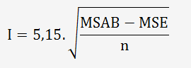
Repeatability and reproducibility are calculated using the following formula:

The variability associated with the part is given by the formula:
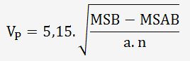
The total variation is obtained by quadratically combining the variability of the measurement system and the variability of the part:


Three operators, OP1, OP2, and OP3, measure a 45 mm dimension L using a calibrated traceable caliper. The tolerance for the dimension is ±1 mm.
| Measurement number |
OP1 |
x̄
|
R1 |
OP2 |
x̄ |
R2 |
OP3 |
x̄ |
R3 |
 |
R̄ |
||||||
| 1 |
45,08 |
45,10 |
45,09 |
45,09 |
0,02 |
45,01 |
45,04 |
45,02 |
45,02 |
0,03 |
45,04 |
45,07 |
45,07 |
45,06 |
0,03 |
45,06 |
0,027 |
| 2 |
44,94 |
44,97 |
44,93 |
44,95 |
0,04 |
44,92 |
44,95 |
44,95 |
44,94 |
0,03 |
44,92 |
44,97 |
44,91 |
44,93 |
0,06 |
44,94 |
0,043 |
| 3 |
45,08 |
45,11 |
45,13 |
45,11 |
0,05 |
44,95 |
45,11 |
45,11 |
45,06 |
0,16 |
45,10 |
45,12 |
45,11 |
45,11 |
0,02 |
45,09 |
0,077 |
| 4 |
44,97 |
45,02 |
45,01 |
45,00 |
0,05 |
45,01 |
44,93 |
45,00 |
44,98 |
0,08 |
45,02 |
44,99 |
44,99 |
45,00 |
0,03 |
44,99 |
0,053 |
| 5 |
44,92 |
44,95 |
45,01 |
44,96 |
0,09 |
44,95 |
44,99 |
44,97 |
44,97 |
0,04 |
44,99 |
44,97 |
44,95 |
44,97 |
0,04 |
44,97 |
0,057 |
| 6 |
45,03 |
45,06 |
45,05 |
45,05 |
0,03 |
45,04 |
45,06 |
44,99 |
45,03 |
0,07 |
45,07 |
45,03 |
45,02 |
45,04 |
0,05 |
45,04 |
0,050 |
| 7 |
45,24 |
45,36 |
45,31 |
45,30 |
0,12 |
45,12 |
45,21 |
45,32 |
45,22 |
0,20 |
45,26 |
45,29 |
45,28 |
45,28 |
0,03 |
45,27 |
0,117 |
| 8 |
45,16 |
45,16 |
45,10 |
45,14 |
0,06 |
45,12 |
45,13 |
45,13 |
45,13 |
0,01 |
45,13 |
45,13 |
45,14 |
45,13 |
0,01 |
45,13 |
0,027 |
| 9 |
45,20 |
45,20 |
45,24 |
45,21 |
0,04 |
45,06 |
45,19 |
45,24 |
45,16 |
0,18 |
45,19 |
45,17 |
45,16 |
45,17 |
0,03 |
45,18 |
0,083 |
| 10 |
45,07 |
45,10 |
45,05 |
45,07 |
0,05 |
45,02 |
45,05 |
45,09 |
45,05 |
0,07 |
45,10 |
45,10 |
45,09 |
45,10 |
0,01 |
45,07 |
0,043 |
| 45,09 |
0,055 |
|
45,06 |
0,087 |
45,08 |
0,031 |
|||||||||||
|
|
R̄1 |
|
R̄2 |
|
R̄3 |
||||||||||||
|
Overall average |
|
45,07 |
 |
0,058
|
|||||||||||||
SSA Calculation:
The sum of all OP1 values is: 1,352.64
The sum of all OP2 values is: 1,351.68
The sum of all OP3 values is: 1,352.38
The sum of all values for the 3 operators is: 4,056.70
b = 10, n = 3, and N = 90
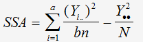

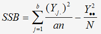
SSB Calculation:
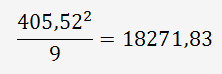
The average squared sum of the 9 measurements (3 operators) for part No. 1 is :
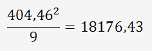
The average squared sum of the 9 measurements (3 operators) for part No. 2 is :
------------------
N°3 : 18298,87 ; N°4 : 18219,60 ; N°5 : 18198,01 ; N°6 : 18256,51
; N°7 : 18440,73 ; N°8 : 18333,16 ; N°9 : 18373,80
------------------
The average squared sum of the 9 measurements (3 operators) for part No. 10 is :
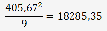
The total amount for the 10 parts is :
18271,83 + 18176,43 + 18298,87 + 18219,60 + 18198,01 + 18256,51
+ 18440,73 + 18333,16 + 18373,80 + 18285,35 = 182854,3082

SSAB Calculation:
The mean square based on the three trials for each operator-part combination is :
Part N°1/OP1 : (45,08 + 45,10 + 45,09)²/3
= 6099,32
Part N°2/OP1 : (44,94 + 44,97 + 44,93)²/3 = 6060,61
Part N°3/OP1 : 6103,83
Part N°4/OP1 : 6075,00
Part N°5/OP1 : 6064,20
Part N°6/OP1 : 6087,61
Part N°7/OP1 : 6151,18
Part N°8/OP1 : 6112,86
Part N°9/OP1 : 6132,74
Part N°10/OP1 : 6094,82
Part N°1/OP2 : 6081,30
Part N°2/OP2 : 6058,81
Part N°3/OP2 : 6090,31
Part N°4/OP2 : 6069,30
Part N°5/OP2 : 6066,90
Part N°6/OP2 : 6083,10
Part N°7/OP2 : 6133,64
Part N°8/OP2 : 6109,25
Part N°9/OP2 : 6119,18
Part N°10/OP2 : 6089,40
Part N°1/OP3 : 6091,21
Part N°2/OP3 : 6057,01
Part N°3/OP3 : 6104,74
Part N°4/OP3 : 6075,00
Part N°5/OP3 : 6066,90
Part N°6/OP3 : 6085,80
Part N°7/OP3 : 6149,93
Part N°8/OP3 : 6111,05
Part N°9/OP3 : 6121,89
Part N°10/OP3 : 6101,13
The total amount is: 182854,3411


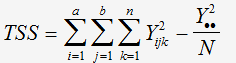
TSS Calculation:
The sum of the squares of all values obtained by the three operators= 182854,4334

SSE Calculation:

SSE = 0,934622 - 0,016435 - 0,80944 - 0,016408 = 0,09234
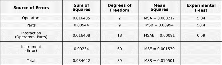
The F-test value must be compared with the critical value provided by the
Fisher-Snedecor F-distribution table for a significance level of α = 0.05.
This distribution, or its inverse, is directly available in Excel® and is
based on the degrees of freedom of the variances:
For example, for: F = MSA / MSE Critical F value = F.INV.RT(0.05,2,60) = 3.12
Since 5.34 > 3.12
Significant: YES
The null hypothesis cannot be accepted.
For: F = MSB / MSE Critical F value = F.INV.RT(0.05,9,60) = 2.04 Since 58.4
> 2.04
Significant: YES
The null hypothesis cannot be accepted.
For: F = MSAB / MSE Critical F value = F.INV.RT(0.05,18,60) = 1.78 Since
0.59 < 1.78
Significant: NO
The null hypothesis can be accepted.
The second table is a “reduced” ANOVA, or an ANOVA recalculated after pooling
the interaction term with the error term.
The Operators × Parts interaction is not significant because its mean square is even lower than the experimental error mean square.
This means that there is no evidence that the operators behave differently depending on the parts. In other words, the interaction is considered negligible.
The non-significant interaction is pooled with the experimental error.
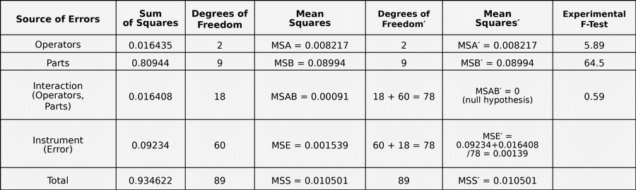
F = MSA' / MSE'
F-test = F.INV.RT(0.05, 2, 78) = 3.11 < 5.89
Significant: YES — the null hypothesis is rejected.
F = MSB' / MSE'
F-test = F.INV.RT(0.05, 9, 78) = 2.00 < 64.5
Significant: YES — the null hypothesis is rejected.
F = MSAB / MSE
F-test = F.INV.RT(0.05, 18, 60) = 1.78 > 0.59
Significant: NO — the null hypothesis is not rejected.
P-value calculations:
Experimental F value = 64.5, degrees of freedom for SSB = 9, and degrees of freedom for SSE' = 78
For Parts: p-value = F.DIST.RT(64.5, 9, 78) ≈ 0.000
Experimental F value = 5.89, degrees of freedom for SSA = 2, and degrees of freedom for SSE' = 78
For Operators: p-value = F.DIST.RT(5.89, 2, 78) = 0.004
Experimental F value = 0.59, degrees of freedom for SSAB = 18, and degrees of freedom for MSE = 60
Part/Operator Interaction: p-value = F.DIST.RT(0.59, 18, 60) = 0.891
Significant effects:
Parts = YES, because 64.5 > 2.00
Operators = YES, because 5.89 > 3.11
Part/Operator Interaction = NO, because 0.59 < 1.78
Let’s calculate the measurement system repeatability, also known as Equipment Variation (EV):

Let’s calculate the measurement system reproducibility (AV):

Let’s calculate the operator-by-part interaction:

Let’s perform the Gage R&R calculation:

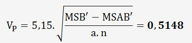
Let’s calculate the part-to-part variability:
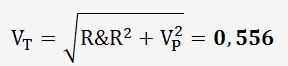
Let’s calculate the total variability:
We then determine the percentage contributions :
%EV = (EV / TV) × 100 = (0.192 / 0.556) × 100 = 34.5% (Equipment)
%AV = (AV / TV) × 100 = (0.0852 / 0.556) × 100 = 15.3% (Operator)
%R&R = (R&R / TV) × 100 = (0.21 / 0.556) × 100 = 37.8%
%Interaction = (0 / 0.556) × 100 = 0% (Part/Operator)
%VP = (PV / TV) × 100 = (0.5148 / 0.556) × 100 = 92.6% (Part)
If the R&R percentage is:
< 10%: the process is satisfactory.
Between 10% and 30%: the process is acceptable, but could
be improved.
> 30%: the process is unacceptable, which is the case
here.
In this case, the process is degraded by operator repeatability, which is
not optimal.
This may be explained by an instrument that is not well suited to the type of dimension being measured, or by a measurement method that does not allow for repeatable results, such as a complex-shaped area or imprecise positioning of the instrument.
If the analysis is focused on the Product, the Tolerance is used instead of the Total Variation.
Both approaches, Total Variation and Tolerance, are valid. The choice depends on how the measurement system is used and on the customer’s requirements.
When the analysis is based on Total Variation, it must be ensured that the measured parts properly represent the Total Process Variation.
Tolerance = IT = 2
%TOL EV = (0.192 / 2) × 100 = 9.6%
%TOL AV = (0.0852 / 2) × 100 = 4.3%
%R&R = (0.21 / 2) × 100 = 10.5%
%Interaction = (0 / 2) × 100 = 0%
%PV = (0.5148 / 2) × 100 = 25.7%
In the present case, the product analysis is acceptable.