
The VIM
The VIM titled JCGM200 published by the BIPM is based on measurement modeling concepts.
In accordance with the GUM and the VIM, a measurement result is generally expressed by two values: a measured value and its associated standard uncertainty.
The measured value and its standard uncertainty represent a range of values attributed to the measurand.
Assume that [x1, u(x1)], ..., [xn, u(xn)] are the results of n different measurements for a measurand considered sufficiently stable, where x1, ..., xn are the measured values and u(x1), ..., u(xn) are the corresponding standard uncertainties.
Within the GUM uncertainty concept, a measured value xi and its associated standard uncertainty u(xi) are considered, respectively, as the probable value, that is, the mathematical expectation E(Xi), and the standard deviation of the probability density function whose knowledge is not completely determined and which is attributed to the measurand for i = 1, ..., n.
The VIM introduces the concept of metrological compatibility, which applies
only to measurement results that are metrologically comparable.
A measured value must be attributable to a recognized metrological reference.
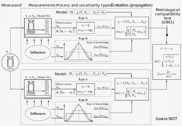
We assume that all results [x₁, u(x₁)], ..., [xn, u(xn)] for a common measurand are traceable to the same metrological reference and are therefore metrologically comparable.
The measured value xi is considered to be the expected value E(Xi), and its standard uncertainty u(xi) is considered to be the standard deviation S(Xi) of the probability density function of Xi for i = 1, 2, j, ..., n.
The difference X₁ − Xⱼ is a variable resulting from the difference between the values assigned by the two results [x₁, u(x₁)] and [xⱼ, u(xⱼ)] to the common measurand.
The expected value and the standard deviation of the probability density
function of (X₁ − Xⱼ) are, respectively:
E(X₁ − Xⱼ) = x₁ − xⱼ and S(X₁ − Xⱼ) = √[u²(x₁) + u²(xⱼ) − 2r(x₁, xⱼ) u(x₁)
u(xⱼ)] where r(x₁, xⱼ) is the correlation coefficient between X₁ and Xⱼ.
According to the VIM, two metrologically comparable results [x₁, u(x₁)] and
[xj, u(xj)] for a measurand assumed to be stable are metrologically compatible
if:
|x₁ − xⱼ| ≤ k × u(x₁ − xⱼ) where k is the coverage factor, generally taken
as equal to 2.
With: u(x₁ − xⱼ) = √[u²(x₁) + u²(xⱼ) − 2r(x₁, xⱼ) u(x₁) u(xⱼ)]
r(x₁, xⱼ) represents the correlation coefficient between the data. If r tends toward 1 or −1, the data are strongly correlated. If r = 0, the data are not correlated.
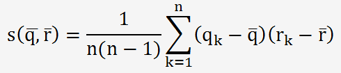 to
estimate the covariance between X₁, denoted q, and Xⱼ, denoted r
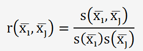 to calculate the correlation coefficient
Supposons n mesures qui donnent des résultats comparables [x1, u(x1)], [xj, u(xj)], ..., [xn, u(xn)], d'un même mesurande mesuré avec une référence certifiée R, ce qui donne le résultat de référence [xR, u(xR)], où xR est la valeur de référence avec une incertitude type u(xR).
On comprend aisément que pour tracer une courbe d'étalonnage et calculer l'incertitude de la relation Y = F(X) en tout point et avec des fonctions autre que linéaires (polynômes de degré 2, 3 ou 4), soit on se contentera d'une pseudo droite Y= ax+b et il est fort probable que notre valeur ne soit pas fiable et peu réaliste soit on utilisera une méthode plus puissante avec un algorithme approprié : Monte Carlo simulation (MCS).
It will allow us to simulate a very large number of values (1,000,000) around a given point, for each point, and to build as many curves as needed: Y1 = F(X1), ... Yn = F(Xn).
Of course, the relationship Y = F(X) will need to be modeled.
Since the equations themselves are affected by error, ε (the residual) is defined as the difference between Y1 and Yn.

Numerical example:
Let’s revisit the graphical example from the datasheet.: Slope and uncertainty of a linear fit on a graph
An unknown solution was titrated with a reagent, and the values were recorded in mV.

Suppose that this time we have standard solutions that already contain the titrant volume, and that each solution is assigned a theoretical potential in mV with an associated expanded uncertainty.
In this specific case, there is no longer any titration involved, but rather a calibration of the titrator through simple measurements at different concentrations.
The uncertainty of the solutions follows a normal distribution (k = 2), while the measurement error follows a rectangular distribution (±2% of the reading).
The weighting represents the relative importance of one uncertainty component, U1, compared with the other components U2, U3, ..., Un.
It is calculated using the formula:
The choice of the polynomial degree can first be tested in Excel. Degrees higher than 2 or 3 force the curve to pass through more points, making it no longer representative between the points.
The Monte Carlo simulation is performed using software that generates the polynomial coefficients, with a second-degree polynomial selected.
| i |
a |
u(a) |
| 0 |
7,387 |
3,782 |
| 1 |
0,902 |
0,0573 |
| 2 |
0,000277 |
0,000184 |
The values have been intentionally rounded.
| r |
a0 |
a1 |
a2 |
| a0 |
1 |
-0,977 |
0,935 |
| a1 |
-0,977 |
1 |
-0,983 |
| a2 |
0,935 |
-0,983 |
1 |
The coefficients appear to be strongly correlated.
The mean residual estimated using the Monte Carlo method is : ε =
-0,102.
The standard uncertainty for this value is : u(ε) = 3,227.
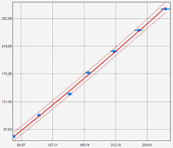
For a reading of 150 mV with an associated error of ±2%, the value is Y = 148.9 mV, with U = ±4.5 mV and k = 2.