
Slope and Uncertainty
Calculating a slope “m” and determining the value of the y-intercept “b” are relatively simple operations.
Y = mx+b
Here are the steps to follow to determine the uncertainty of a Y value as a function of x, the slope “m,” and the y-intercept “b.”
We consider a graph (x, Y) made up of 7 distinct points.
Let us take a concrete example: the titration of a given solution with a reagent, where x is the volume of titrant added in mL and Y is the electrode response in mV.
For now, we are looking for the uncertainty on Y when x = 2.2 mL.
Each data point, both input and result, has been assigned its own uncertainty.
| Data |
Y |
X |
| Unity | mV | ml |
| U | ± 10 | ± 0,2 |
| 1 |
75 | 1,0 |
| 2 |
109 | 1,5 |
| 3 | 150 | 2,0 |
| 4 | 175 | 2,5 |
| 5 | 210 | 3,0 |
| 6 | 243 | 3,5 |
| 7 | 279 | 4,0 |
We will indicate the total uncertainty of each point on the graph.
To do this, draw one vertical line and two horizontal lines, with half-lengths
equal to the uncertainties.
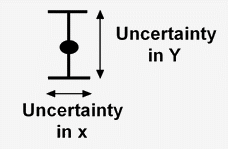
These lines define what is known as an “uncertainty rectangle.”
Draw the best-fit line through all the points (using Excel is practical). Note that the extreme points pass through the best-fit line; if this is not the case, see the NOTE.
Draw two lines: the first passing above the values and through the upper corners of the extreme uncertainty rectangles, and the second passing below the values and through the lower corners (blue lines).

This “tunnel” technique on the graph corresponds to interpolation, meaning
the determination of a value located within the range covered by the measurements.
NOTE 2
Calculate the two slopes, “m1” and “m2”.

m1 = m2 = 68
m
m
For x = 2.2 ± 0.2 mL, the Y values are graphically determined for x = 2.0 mL and 2.4 mL.
The following values are obtained: Y = 120 and 167 mV for x = 2.0 mL, and Y = 147 and 194 mV for x = 2.4 mL.
Calculation of Y
Calculation of U = [(194 + 167) / 2 − (147 + 120) / 2] = ±23.5 mV
Y = (157,0 ± 23,5) mV: This technique necessarily leads to a conservative uncertainty estimate. (see the least-squares method).
To determine the uncertainty on the slope, the “X” technique must be used.
These lines must pass through all the uncertainty rectangles.
Using the same coordinates as for the previous points, the minimum slope
m
Maximum coordinates: (289; 3.8) and (65; 1.2)
Minimum coordinates: (269; 4.2) and (85; 0.8)
Equation 1: m
Calculation of m
Calculation of U on m
m
If there is no singular point (NOTE 3), the value from the Excel trendline
will be used: m
m
To calculate the uncertainty on the intercept b, we will use a remarkable point ((x_c; Y_c = 2.5; 177.5)) through which the three lines pass, as shown on the graph.
Since the measurement of (x_c) on the graph is not very precise, use the Excel trendline to determine this point accurately.
We can write:
Yc = m
Yc = m
Yc = m

By applying this equation, this amounts to writing that:
Delta (b) = U.xc = 16 . 2,5 = ± 40.
b
b
It can be observed that if b
If the graph is plotted on a semi-logarithmic scale: see NOTES.

1 - On the graph, if one of the end points does not lie on the best-fit line,
draw an uncertainty rectangle of the same size near the point and centered
on the line.
One can be drawn at each end if the best-fit line does not pass through either
end point.
2 - If the value being sought lies outside the measurement range, extrapolation
will be performed using an “X” technique, shown as dashed lines on the graph.
A first line is drawn with the steepest possible slope, “m
3 - A value is considered “singular” when it does not follow the natural trend
of the line or curve: erroneous value, incorrect handling, normal phenomenon
but insufficient resolution; in this case, repeat the measurements with more
points around the problematic area.
4 - In the case of a semi-logarithmic graph:
