Control Limits in Control Charts
There is a right way—and a wrong way—to calculate control chart limits.
Do you know the difference?
story:
It is 1930, and a senior executive asks his team leader, Paul, to use a control chart to monitor production in the factory.
Paul did not know where to begin, so he asked himself what data he should collect. After thinking it over, he decided he could start with data that were already known in the factory.
Paul therefore began his data collection with a log sheet on which he recorded the previous week’s production.
On the log sheet, he wrote down the weight of each batch manufactured by the production operators.
Paul plotted the batch weights on a piece of graph paper, and after filling
the first page, he calculated the limits for an individual values chart, also
known as an XmR chart: individual value X and moving range mR.
Of course, the process was out of control and unpredictable.
Even though each batch had been weighed, and even though the operators had written down every one of those weights, the chart could not help them produce batches with consistent weights. The unpredictable weights meant that the formulation was changing unpredictably, which led to a sense of fatalism, because some days the weights had been better than others, and there was nothing he could do about it.
How could Paul determine that the process was unpredictable? The answer lies in the way the limits are calculated. We will now look at how Paul performed his calculations.
Below are the production results, in kg, over a 20-day period
| 920 |
925 |
830 |
855 |
905 |
| 925 |
945 |
915 |
940 |
940 |
| 910 |
860 |
865 |
985 |
970 |
| 940 |
970 |
1000 |
1035 |
1040 |
The first step is to determine the centerline of the chart, which is generally the average of the individual values. For these 20 values, the average is 934.
There are two methods for calculating the limits of the XmR control chart after the centerline has been determined. Paul calculates the moving ranges.
The moving ranges are the differences between successive values.
For the first data pair in the range, the range is 925 to 920 = 5.
The second pair is 830 to 925 = -95. However, by convention, moving ranges are always positive. Paul therefore drops the negative sign and obtains a moving range of 95. For the 20 data points above, the 19 moving ranges are as follows:
| / |
5 |
95 |
25 |
50 |
| 20 |
20 |
30 |
25 |
0 |
| 30 |
50 |
5 |
120 |
15 |
| 30 |
30 |
30 |
35 |
5 |
With a center line and a set of moving ranges, Paul is now ready to calculate the limits using one of two methods.
A first correct method:
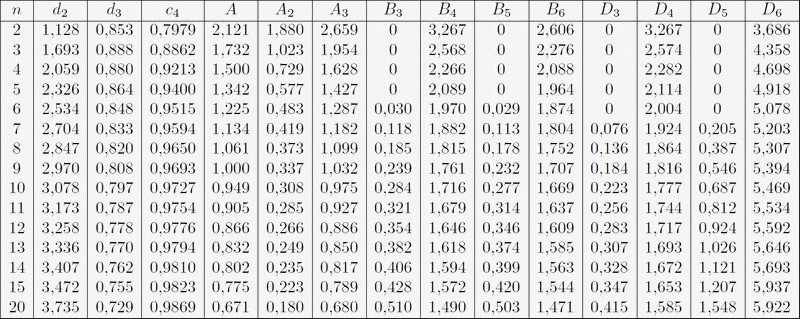
See the Burr constants table at the bottom of the page.
The most common method for determining limits for XmR charts is to use the average moving ranges, which are commonly denoted by the symbol: Rbar.
The chart limits are determined by multiplying the average moving range
(32.63) by the constant A3 = 2.66 (= 3 / (d
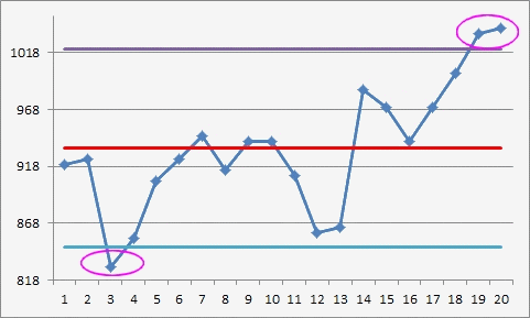
Xbar − 2.66Rbar and Xbar + 2.66Rbar, with 2.66Rbar = 32.63 × 2.66 = 86.8, giving a lower limit of 847.2 and an upper limit of 1020.8.
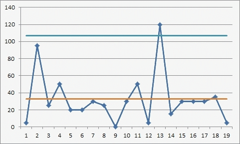
The upper limit for the range chart is obtained by multiplying the average
moving range by the constant 3.267 (D
A second valid method:
It consists of calculating the control chart limits for a table of individual values using the median moving range (25) for the 19 values. To determine the median of a set of values, simply arrange the values in ascending order and select the value located at the center of the list. This is commonly denoted by the symbol:

The chart limits can be found by multiplying the median moving range by the constant 3.145, then adding and subtracting this product from the average.
By multiplying:
.=
Multiplying 25 by the constant 3.145 gives 78.625. The control chart limits
are therefore:
X̄ − 78.625 and X̄ + 78.625, i.e. Lower Limit = 855.4 and Upper Limit = 1012.6
The upper limit for the range chart is obtained by multiplying the median moving range by the constant 3.865. For these data, this limit is 96.6 = 3.865 × 25.
These limits are slightly narrower than those calculated using the first method, and the chart will now have a fourth point outside the limits: the value 855.
There is no practical difference between these two methods for calculating the limits.
An Incorrect Method:
This method should only be used when the variability is controlled and properly bounded.
A common but incorrect method for calculating control chart limits is to use a measure of variability calculated from all the data. For example, the 20 data points could be used to calculate a standard deviation. The common symbol for this statistic is the lowercase letter s. For these 20 data points:
s = 56,5
The 3-sigma limits are then mistakenly calculated as mean + 3σ::
934 ± 170 soit Lower Limit = 764 et Upper Limit = 1104
Using appropriate methods to calculate the limits makes it possible to detect alerts in the data, even though the data used in the calculations include alerts. Correct methods are always based on an average value or a median measure of dispersion.
Incorrect methods will inevitably limit the alerts present in the data and therefore mask the problems.
Incorrect methods tend to rely on a single measure of dispersion, calculated using all of the data.
If you want to use a standard deviation, please refer to the relevant sheet.: "Choosing Control Limits for Control Charts"